本文共 5662 字,大约阅读时间需要 18 分钟。
0:环境
本教程的环境是Python2.7、Keras+Tensorflow、sklearn、matplotlib、numpy
Ubuntu18.
1:原理
LeNet结构是LeCun在1998年提出了神经网络结构。本结构在OCR文字识别方面有较大优势,识别精度较高。
网络的结构是:INPUT => CONV => ACT => POOL => CONV => ACT => POOL => FC => ACT => FC => SOFTMAX
见下表:
| Layer Type | Output Size | Filter Size / Stride |
| INPUT IMAGE | 28 x 28 x 1 | |
| CONV | 28 x 28 x 20 | 5 x 5, K = 20 |
| ACT | 28 x 28 x 20 | |
| POOL | 14 x 14 x 20 | 2 x 2 |
| CONV | 14 x 14 x 50 | 5 x 5, K = 50 |
| ACT | 14 x 14 x 50 | |
| POOL | 7 x 7 x 50 | 2 x 2 |
| FC | 500 | |
| ACT | 500 | |
| FC | 10 | |
| SOFTMAX | 10 |
输入层是28 x 28 x 1的黑白图片。
第二层是 28 x 28 x 20的大小,生成方式是使用20个5 x 5的filter分别对输入图片进行卷积。与神经网络类似,每个点都有自身的激活函数。同时带有POOLING(池化层),本层的Filter矩阵是2 x 2。每2 x 2之间只留下一个最大值自上到下从左到右的处理,POOL的输出尺寸只有输入的1/4大小。
第三层也是CONV + ACT + POOL的形式。
第四层是全连接的500个神经元。全连接的意思是,第三层的全部输入都分别和第四层的每个神经元相连。假如不说明FC,则默认两层之间的连接线,有一定概率会失去连接。
第五层是输出层。
2:代码
有两个文件,分别是lenet.py和lenet_mnist.py。放在同一个目录即可。
2.1 lenet.py
# import the necessary packagesfrom keras.models import Sequentialfrom keras.layers.convolutional import Conv2Dfrom keras.layers.convolutional import MaxPooling2Dfrom keras.layers.core import Activationfrom keras.layers.core import Flattenfrom keras.layers.core import Densefrom keras import backend as Kclass LeNet: @staticmethod def build(width, height, depth, classes): # initialize the model model = Sequential() inputShape = (height, width, depth) # if we are using "channels first", update the input shape if K.image_data_format() == "channels_first": inputShape = (depth, height, width) # first set of CONV => RELU => POOL layers model.add(Conv2D(20, (5, 5), padding="same", input_shape=inputShape)) model.add(Activation("relu")) model.add(MaxPooling2D(pool_size=(2, 2), strides=(2, 2))) # second set of CONV => RELU => POOL layers model.add(Conv2D(50, (5, 5), padding="same")) model.add(Activation("relu")) model.add(MaxPooling2D(pool_size=(2, 2), strides=(2, 2))) # first (and only) set of FC => RELU layers model.add(Flatten()) model.add(Dense(500)) model.add(Activation("relu")) # softmax classifier model.add(Dense(classes)) model.add(Activation("softmax")) # return the constructed network architecture return model 2.2 lenet_mnist.py
# import the necessary packagesfrom lenet import LeNetfrom keras.optimizers import SGDfrom sklearn.preprocessing import LabelBinarizerfrom sklearn.model_selection import train_test_splitfrom sklearn.metrics import classification_reportfrom sklearn import datasetsfrom keras import backend as Kimport matplotlib.pyplot as pltimport numpy as npimport os# grab the MNIST dataset (if this is your first time using this# dataset then the 55MB download may take a minute)print("[INFO] accessing MNIST...")#dataset = datasets.fetch_mldata("MNIST Original")path1 = os.path.dirname(os.path.abspath(__file__))dataset = datasets.fetch_mldata("MNIST Original", data_home=path1)data = dataset.data# if we are using "channels first" ordering, then reshape the# design matrix such that the matrix is:# num_samples x depth x rows x columnsif K.image_data_format() == "channels_first": data = data.reshape(data.shape[0], 1, 28, 28) # otherwise, we are using "channels last" ordering, so the design# matrix shape should be: num_samples x rows x columns x depthelse: data = data.reshape(data.shape[0], 28, 28, 1)# scale the input data to the range [0, 1] and perform a train/test# split(trainX, testX, trainY, testY) = train_test_split(data / 255.0, dataset.target.astype("int"), test_size=0.25, random_state=42) # convert the labels from integers to vectorsle = LabelBinarizer()trainY = le.fit_transform(trainY)testY = le.transform(testY)# initialize the optimizer and modelprint("[INFO] compiling model...")opt = SGD(lr=0.01)model = LeNet.build(width=28, height=28, depth=1, classes=10)model.compile(loss="categorical_crossentropy", optimizer=opt, metrics=["accuracy"])# train the networkprint("[INFO] training network...")H = model.fit(trainX, trainY, validation_data=(testX, testY), batch_size=128, epochs=20, verbose=1)# evaluate the networkprint("[INFO] evaluating network...")predictions = model.predict(testX, batch_size=128)print(classification_report(testY.argmax(axis=1), predictions.argmax(axis=1), target_names=[str(x) for x in le.classes_]))# plot the training loss and accuracyplt.style.use("ggplot")plt.figure()plt.plot(np.arange(0, 20), H.history["loss"], label="train_loss")plt.plot(np.arange(0, 20), H.history["val_loss"], label="val_loss")plt.plot(np.arange(0, 20), H.history["acc"], label="train_acc")plt.plot(np.arange(0, 20), H.history["val_acc"], label="val_acc")plt.title("Training Loss and Accuracy")plt.xlabel("Epoch #")plt.ylabel("Loss/Accuracy")plt.legend()plt.show() 初次运行以下代码,初次调用sklearn的fetch_mldata会在本文件的目录内生成mldata文件夹,并把MNIST的dataset下载到该目录内。只有50多MB,但是速度和机器性能、网络有关。
path1 = os.path.dirname(os.path.abspath(__file__))dataset = datasets.fetch_mldata("MNIST Original", data_home=path1) 3:运行结果
[INFO] evaluating network... precision recall f1-score support 0 0.99 0.99 0.99 1677 1 0.99 0.99 0.99 1935 2 0.98 0.99 0.98 1767 3 0.99 0.97 0.98 1766 4 0.98 0.99 0.99 1691 5 0.99 0.97 0.98 1653 6 0.99 0.99 0.99 1754 7 0.99 0.98 0.98 1846 8 0.94 0.98 0.96 1702 9 0.98 0.97 0.98 1709avg / total 0.98 0.98 0.98 17500
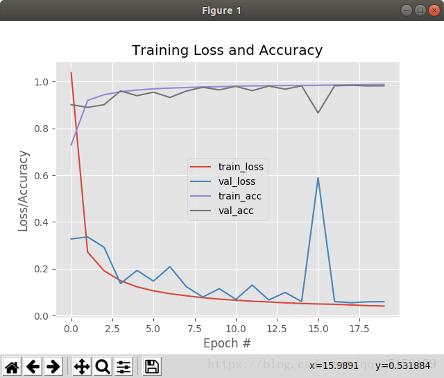
可以达到98%的精度,数据十分可观。
我的电脑是i3-6100的CPU,需要90秒才能完成一次迭代,没有GPU。书本的作者的CPU要30秒,GPU只要3秒。
所以,TODO:在GPU上跑
参考资料(也是代码来源):Deep.Learning.for.Computer.Vision.with.Python.Starter.Bundle.pdf